You can find a repository of good solutions to the book exercises here.
Building Abstractions with Procedures
The Elements of Programming
A programming language is our mental framework for organising ideas about process. It provides three mechanisms for combining simple ideas such that they together form more complex ideas:
- primitive expressions, which represent the simplest entities the language is concerned with,
- means of combination, by which compound elements are built from simpler ones, and
- means of abstraction, by which compound elements can be named and manipulated as units.
Expressions
Expressions such as these, formed by delimiting a list of expressions within parentheses in order to denote procedure application, are called combinations. the leftmost element in the list is called the operator , and the other elements are called operands . The value of a combination is obtained by applying the procedure specified by the operator to the arguments that are the values of the operands.
Placing the operator to the left of the operands is called prefix-notation.
Let’s take a look at the nesting of expressions:
(+ (* 3
      (+ (* 2 4)
         (+ 3 5)))
   (+ (- 10 7)
      6))
If we align the operands vertically as above we pretty-print our code.
Naming and the Environment
Every programming language uses names which identify a variable whose
value is the object. In the Scheme dialect of list we use define. In Lisp
every expression has a value.
Lisp programmers know the value of everything but the cost of nothing (Alan Perlis)
Here is an example of how to use define:
(define pi 3.14159)
(define radius 10)
(* pi (* radius radius))

(define circumference (* 2 pi radius))
circumference
In order to keep track of the name-object pairs, the interpreter maintains a memory called the (global) environment.
Evaluating Combinations
Let us consider the following recursive evaluation rule:
To evaluate a combination, do the following:
- Evaluate the subexpressions of the combination.
- Apply the procedure that is the value of the leftmost subexpression (the operator) to the arguments that are the values of the other subexpressions (the operands).
Hence, the following code
(* (+ 2 (* 4 6))
   (+ 3 5 7))
can be represented in the following tree strucure:
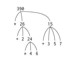
This “percolating upwards” is called tree accumulation. This evaluation rule
does not apply to so-called special forms, such as define, which each have
their own evaluation rule.
Compound Procedures
Any programming language must have:
- Numbers and arithmetic operations are primitive data and procedures. Nesting
- of combinations provides a means of combining opera- tions. Definitions that
- associate names with values provide a limited means of abstraction.
Next, we need procedure definitions which open a whole new realm of possibility.
Let’s define a compound procedure called square:
(define (square x) (* x x))Now we can easily define another procedure that makes use of square:
(define (square x) (* x x))
(define (sum-of-squares x y)
  (+ (square x) (square y)))
(sum-of-squares 3 4)
which evaluates to 25. We can take this even further:
(define (square x) (* x x))
(define (sum-of-squares x y)
  (+ (square x) (square y)))
(define (f a)
  (sum-of-squares (+ a 1) (* a 2)))
(f 5)
which gives us 136.
The Substitution Model for Procedure Application
Let us consider the combination from above to illustrate the subsitution model:
(f 5)
;; retrieve the body of f and replace parameters with the arguments
(sum-of-squares (+ 5 1) (* 5 2))
;; apply sum-of-square to 6 and 10
(+ (square 6) (square 10))
;; reduce the expression by using the definition of square
(+ (* 6 6) (* 10 10))
(+ 36 100)NB: This is not how the interpreter really works, as we’ll see later. The subsitution model serves the purpose of providing an entry point to thinking about procedure application.
Applicative vs. Normal Order
The “first evaluate arguments and then apply procedures” way of doing things that we used above (applicative-order evaluation) is not the only way.
The other evaluation model is the “fully expand and then reduce” model, which is called normal-order evaluation and illustrated below:
(f 5)
(sum-of-squares (+ 5 1) (* 5 2))
(+    (square (+ 5 1))      (square (* 5 2))  )
(+    (* (+ 5 1) (+ 5 1))   (* (* 5 2) (* 5 2)))
(+         (* 6 6)             (* 10 10))
(+           36                   100)
                    136
Conditional Expression and Predicates
Often, we want to do different things depending on the result of a test (case
analysis). In Lisp we use cond to do that. The first expression in each pair
is called the predicate (either true or false) and the second one is the
consequent expression (value returned if predicate is true).
(define (abs x)
;;      (<p>   <e>)
  (cond ((> x 0) x)
        ((= x 0) 0)
        ((< x 0) (- x))))

;; use else when to specify what to return if all clauses have been bypassed
(define (abs x)
  (cond ((< x 0) (- x))
        (else x)))

;; use if if you have exactly two cases in the case analysis
(define (abs x)
  (if (< x 0)
      (- x)
      x))
Of course, we should be able to construct compound predicates also with logical composition operations and not purely numerical ones:
;; specify a number range: 5 < y < 10
(and (> x 5) (< x 10))

;; greater than or equal
(define (>= x y)
  (or (> x y) (= x y)))

;; alternatively:
(define (>= x y)
  (not (< x y)))
Exercise 1.1
Below is a sequence of expressions. What is the result printed by the interpreter in response to each expression? Assume that the sequence is to be evaluated in the order in which it is presented.
10
;; 10
(+ 5 3 4)
;; 12
(- 9 1)
;; 8
(/ 6 2)
;; 3
(+ (* 2 4) (- 4 6))
;; 6
(define a 3)
;; a
(define b (+ a 1))
;; b
(+ a b (* a b))
;; 19
(= a b)
;; #f
(if (and (> b a) (< b (* a b)))
    b
    a)
;; 4
(cond ((= a 4) 6)
      ((= b 4) (+ 6 7 a))
      (else 25))
;; 16
(+ 2 (if (> b a) b a))
;; 6
(* (cond ((> a b) a)
         ((< a b) b)
	     (else -1))
   (+ a 1))
;; 16
Exercise 1.2
Translate the following expression into prefix form:
(/ (+ 5 4
      (- 2
         (- 3
            (+ 6
               (/ 4 5)))))
   (* 3
      (- 6 2)
      (- 2 7)))
;; -37/150
Exercise 1.3
Define a procedure that takes three numbers as arguments and returns the sum of the squares of the two larger numbers.
(define (sq x)
  (* x x))

(define (ssq x y)
  (+ (sq x) (sq y)))

(define (max3 x y z)
  (cond ((> x y) (cond ((> x z) x)
                       (z)))
        ((> y z) y)
         (z)))

(define (max2 x y)
  (if (> x y) x y))

(define (larger-ssq x y z)
  (cond ((= (max3 x y z) x) (ssq x (max2 y z)))
        ((= (max3 x y z) y) (ssq y (max2 x z)))
        ((= (max3 x y z) z) (ssq z (max2 x y)))))
Exercise 1.4
Observe that our model of evaluation allows for combinations whose operators are compound expressions. Use this observation to describe the behavior of the following procedure:
(define (a-plus-abs-b a b)
  ;; the if-expression evaluates to a "+" or "-" depending on the clause (> b 0)
  ((if (> b 0) + -) a b))
Exercise 1.5
Ben Bitdiddle has invented a test to determine whether the interpreter he is faced with is using applicative-order evaluation or normal-order evaluation. He defines the following two procedures:
(define (p) (p))
(define (test x y)
  (if (= x 0) 0 y))

(test 0 (p))
Using normal-order evaluation, the last expression evaluates to 0 as the
infinite-loop-producing procedure p is not evaluated. This is not true for
applicative-order evaluation, where the arguments are evaluated first. Here, the
process ends in an infinite loop.
Example: Square Roots by Newton’s Method
There is a difference between a mathematical function of a square root (which can be used to recognise a square root or derive some interesting insights about it) and a procedure to generate a squre root.
For generating sqaure roots, we can use Newton’s method of approximation:
(define (sqrt-iter guess x)
  (if (good-enough? guess x)
      guess
      (sqrt-iter (improve guess x)
                 x)))

(define (improve guess x)
  (average guess (/ x guess)))

(define (average x y)
  (/ (+ x y) 2))

(define (good-enough? guess x)
  (< (abs (- (square guess) x)) 0.001))

(define (sqrt x)
  (sqrt-iter 1.0 x))
The sqrt-iter procedure also underlines that iteration can be achieved using
no special construct but the ability to call a procedure
Exercise 1.6
Alyssa P. Hacker doesn’t see why if needs to be provided as a special form. “Why can’t I just define it as an ordinary procedure in terms of cond ?” she asks. Alyssa’s friend Eva Lu Ator claims this can indeed be done, and she defines a new version of if:
(define (new-if predicate then-clause else-clause)
  (cond (predicate then-clause)
        (else else-clause)))
;; demo
(new-if (= 2 3) 0 5)
;; 5
(new-if (= 1 1) 0 5)
;; 0
Now, Alyssa wants to use new-if for the square-root program:
(define (sqrt-iter guess x)
  (new-if (good-enough? guess x)
          guess
          (sqrt-iter (improve guess x)
                     x)))
What happens when Alyssa aempts to use this to compute square roots? Explain.
The interpreter returns the following error message:
;Aborting!: maximum recursion depth exceeded
This is due to the fact that the new-if procedure does not share the property
of the if special form to only evaluate the consequence when the predicate
evaluates to #t. Hence, infinite recursion whenever we call new-if and there
one of the consequents is a function call.
Exercise 1.7
The good-enough? test used in computing square roots will not be very
effective for finding the square roots of very small numbers. Also, in real
computers, arith- metic operations are almost always performed with lim- ited
precision. this makes our test inadequate for very large numbers. Explain these
statements, with examples showing how the test fails for small and large
numbers. An alternative strategy for implementing good-enough? is to watch how
guess changes from one iteration to the next and to stop when the change is a
very small fraction of the guess. Design a square-root procedure that uses this
kind of end test. Does this work beer for small and large numbers?
(define (sqrt-iter guess x)
  (if (good-enough? guess (improve guess x) x)
      guess
      (sqrt-iter (improve guess x)
                 x)))

(define (abs x)
  (if (< x 0)
      (- x)
      x))

(define (improve guess x)
  (average guess (/ x guess)))

(define (average x y)
  (/ (+ x y) 2))

(define (good-enough? cur next x)
  (< (/ (abs (- cur next)) x) 0.0000001))

(define (sqrt x)
  (sqrt-iter 1.0 x))
Exercise 1.8
Newton’s method for cube roots is based on the fact that if y is an approximation to the cube root of x, then a beer approximation is given by the value
Use this formula to implement a cube-root procedure analogous to the square-root procedure
(define (cbrt-iter guess x)
  (if (good-enough? guess (improve guess x) x)
      guess
      (cbrt-iter (improve guess x)
                 x)))

(define (abs x)
  (if (< x 0)
      (- x)
      x))

(define (square x) (* x x))

(define (improve guess x)
  (/ (+ (/ x (square guess)) (* 2 guess)) 3))

(define (good-enough? cur next x)
  (< (/ (abs (- cur next)) x) 0.0000001))

(define (cbrt x)
  (cbrt-iter 1.0 x))
Procedures as Black-Box Abstractions
The procedure definition binds its formal parameters such that they become bound variables. If variables are not bound, they are free. The set of expressions for which there is a binding defines its name is called scope of that name.
Often it can be useful to “hide” or localise the subprocedures of a given
procedure by utilising what is called a block structure. In the case of our
sqrt function, we could write:
(define (sqrt x)
  (define (good-enough? guess x)
    (< (abs (- (square guess) x)) 0.001))
  (define (improve guess x)
    (average guess (/ x guess)))
  (define (sqrt-iter guess x)
    (if (good-enough? guess x)
        guess
        (sqrt-iter (improve guess x) x)))
  (sqrt-iter 1.0 x))
As can be inspected above, x is a free variable in the internal procedure
definitions. This discipline is called lexical scoping, which the authors
define as follows:
Lexical scoping dictates that free variables in a procedure are taken to refer to bindings made by enclosing procedure definitions; that is, they are looked up in the environment in which the procedure was defined.
Procedures and the Processes They Generate
Our situation is now analogous to someone who knows the rules of how pieces move in chess but knows nothing of openings, tactics or strategy. We don’t know any patterns yet.
A procedure is a pattern for the local evolution of a computational process. It specifies how each stage of the process is built upon the previous stage
Linear Recursion and Iteration
Consider the factorial function:
Another way to write this is:
From the latter, we can define the following procedure to generate the factorial of \(n\):
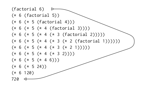
(define (factorial n)
  (if (= n 1)
      1
      (* n (factorial (- n 1)))))
The authors visulise the resulting recursion of \(6!\) as follows:
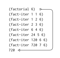
We can also iterate by defining a counter that increases by one each step and is multiplied with the product of the last iteration. So, \(n!\) is the value of the product when the counter exceeds \(n\).
(define (factorial n)
  (define (iter product counter)
    (if (> counter n)
        product
        (iter (* counter product)
              (+ counter 1))))
  (iter 1 1))
This can be visualised as follows:
Here some important distinctions are to be made. The authors clarify that a recursive process is different from a recursive procedure:
When we describe a procedure as recursive, we are referring to the syntactic fact that the procedure definition refers (either directly or indirectly) to the procedure itself. But when we describe a process as following a pattern that is, say, linearly recursive, we are speaking about how the process evolves, not about the syntax of how a procedure is written.
Scheme is tail-recursive, i.e. it executes an iterative process in constant
space, even if it is described by a recursive procedure. This means, that in
Scheme we don’t need any special iteration constructs such as for, while,
until etc. They are only useful as
sytactic sugar.
Exercise 1.9
Each of the following two procedures defines a method for adding two positive
integers in terms of the procedures inc, which increments its argument by 1,
and dec, which decrements its argument by 1.
(define (+ a b)
  (if (= a 0)
      b
      (inc (+ (dec a) b))))

;; (inc (+ 3 5))
;; (inc (inc (+ 5 2)))
;; (inc (inc (inc (+ 1 5))))
;; (inc (inc (inc (inc (+ 0 5)))))
;; (inc (inc (inc (inc (5)))))
;; (inc (inc (inc 6)))
;; (inc (inc 7))
;; (inc 8)
;; 9
;; --> recursive

(define (+ a b)
  (if (= a 0)
      b
      (+ (dec a) (inc b))))

;; (+ 3 6)
;; (+ 2 7)
;; (+ 1 8)
;; (+ 0 9)
;; 9
;; --> iterative process:
Exercise 1.10
The following procedure computes a mathematical function called Ackermann’s
function. What are the values of the expression below the procedure definition.
Also, give concise mathematical definitions for the functions computed by the
procedures f , g , and h for positive integer values of \(n\). For
example, (k n) computes \(5n^2\).
(define (A x y)
  (cond ((= y 0) 0)
        ((= x 0) (* 2 y))
        ((= y 1) 2)
        (else (A (- x 1)
                 (A x (- y 1))))))

(A 1 10)
;; 1024

(A 2 3)
;; 65536

(A 3 3)
;; 65536

(define (f n) (A 0 n))
;; 2n
(define (g n) (A 1 n))
;; 2^n
(define (h n) (A 2 n))
;; 2^2^2^2 : n times
;; Knuth's up-arrow notation
(define (k n) (* 5 n n))
;; 5n^2
Tree Recursion
To understand tree recursion, consider the Fibonacci sequence:
In general, the Fibonacci numbers can be defined by the rule:
Let’s translate that into Lisp:
(define (fib n)
  (cond ((= n 0) 0)
        ((= n 1) 1)
        (else (+ (fib (- n 1))
                 (fib (- n 2))))))
This is pretty bad as the number of times that the procedure will compute is precisely Fib\((n + 1)\), e.g. in the case above exactly eight times. Thus, the process uses a number of steps that grows exponentially with the input. The space, however, only grows linearly with the input as we only need to keep track of the nodes above the current one at any point during computation.
Let’s define an iterative procedure to do the same thing:
(define (fib n)
  (fib-iter 1 0 n))

(define (fib-iter a b count)
  (if (= count 0)
      b
      (fib-iter (+ a b) a (- count 1))))
The authors summarise:
The difference in number of steps required by the two methods — one linear in n, one growing as fast as Fib(n) itself — is enormous, even for small inputs.
However, tree-recursive processes aren’t useless. Often, they are easier to design and understand. Apparently, the Scheme interpreter itself evaluates expression using a tree-recursive process.
Example: Counting Change
(define (count-change amount)
  (cc amount 5))

(define (cc amount kinds-of-coins)
  (cond ((= amount 0) 1)
        ((or (< amount 0) (= kinds-of-coins 0)) 0)
        (else (+ (cc amount
                     (- kinds-of-coins 1))
                 (cc (- amount
                        (first-denomination kinds-of-coins))
                     kinds-of-coins)))))

;; takes kinds of coins available
;; returns denomination of first kind
(define (first-denomination kinds-of-coins)
  (cond ((= kinds-of-coins 1) 1)
        ((= kinds-of-coins 2) 5)
        ((= kinds-of-coins 3) 10)
        ((= kinds-of-coins 4) 25)
        ((= kinds-of-coins 5) 50)))

(count-change 10)
Exercise 1.11
A function f is defined by the rule that
f(n)=\left\\{\begin{array}{ll}n \quad \text { if } n<3 \\ f(n-1)+2 f(n-2)+3 f(n-3) & \text { if } \quad n \geq 3\end{array}\right.Write a procedure that computes \(f\) by means of a recursive process. Write a procedure that computes \(f\) by means of an iterative process.
;; recursive
(define (f-recur n)
  (cond ((< n 3) n)
        (else (+ (f-recur (- n 1))
                 (* 2 (f-recur (- n 2)))
                 (* 3 (f-recur (- n 3)))))))

(f-recur 10)
;; 1892

;; iterative version 1
(define (f-iter-1 n)
  (define (f-iter a b c count)
    (cond ((< count 0) count)
          ((= count 0) a)
          ((= count 1) b)
          ((= count 2) c)
          (else (f-iter b c (+ c (* 2 b) (* 3 a)) (- count 1)))))
  (f-iter 0 1 2 n))

(f-iter-1 4)
;; f-iter (1 2 (+ 2 (* 2 1) (* 3 0)) (- 3 1))
;; f-iter (1 2 (+ 2 2 0)) 2)
;; f-iter (1 2 4 2)
;; --> 4

;; iterative version 2
(define (f-iter-2 n)
  (define (f-iter a b c count)
    (cond ((< n 3) n)
          ((<= count 0) a)
          (else (f-iter (+ a (* 2 b) (* 3 c)) a b (- count 1)))))
  (f-iter 2 1 0 (- n 2)))

(f-iter-2 10)
;; 1892
Exercise 1.12
The following pattern of numbers is called Pascal’s triangle:
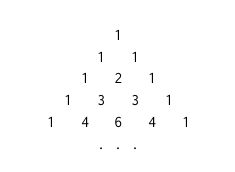
The numbers at the edge of the triangle are all 1, and each number inside the triangle is the sum of the two numbers above it. Write a procedure that computes elements of Pascal’s triangle by means of a recursive process.
(define (pascal r c)
  (if (or (= c 1) (= c r))
       1
       (+ (pascal (- r 1) (- c 1))
          (pascal (- r 1) c))))

(pascal 5 3)
;; 6

;;   c
;; r 1
;;   1 1
;;   1 2 1
;;   1 3 3 1
;;   1 4 6 4 1
;;   ...
Exercise 1.13
-
Proposition
For all \(n \in \mathbb{N}\) let \(P(n)\) be the proposition:
\(Fib(n)=\frac{\varphi^{n}-{\psi}^{n}}{\sqrt{5}}\)
-
Basis for induction
\(P(0)\) is true, as this shows:
-
Induction hypothesis
\(\forall 0 \le j \le k + 1: Fib(j) = \dfrac {\varphi^j - \psi^j} {\sqrt 5}\)
Thus, we need to show:
\(Fib(k + 2) = \dfrac {\varphi^{k + 2} - \psi^{k + 2} } {\sqrt 5}\)
-
Induction step
We have the following two identities:
Hence:
\(= (\varphi^{k}-\psi^{k})+(\varphi^{k+1}-\psi^{k+1})\)
The result follows by the principle of mathematical induction.
Therefore:
\(\forall n \in \mathbb{N}: Fib(n) = \frac {\varphi^n - \psi^n} {\sqrt 5}\)
Orders of Growth
Let \(R(n)\) be the amount of resources the process requires for a problem of size \(n\).
The authors make some further important definitions
We say that \(R(n)\) has order of growth \(\theta(f(n))\), written $R(n) = θ(f(n)) (pronounced “theta of \(f(n)\)”), if there are positive constants \(k_1\) and \(k_2\) independent of \(n\) such that \(k_1f(n) \leq R(n) \leq k_2 f(n)\) for any sufficiently large value of \(n\). (In other words, for large \(n\), the value \(R(n)\) is sandwiched between \(k_1 f (n)\) and \(k_2 f (n)\).)
Exercise 1.14
Draw the tree illustrating the process generated by the aforementioned
count-change procedure of in making change for 11 cents. What are the orders
of growth of the space and number of steps used by this process as the amount to
be changed increases?
(count-change 11)
|
(cc 11 5)__
|          \
(cc 11 4)   (cc -39 5)
|       \___
|           \
(cc 11 3)   (cc -14 4)
|       \_______________________________________________________
|                                                               \
(cc 11 2)                                                      (cc 1 3)
|       \_________________________                              |     \__
|                                 \                             |        \
(cc 11 1)                        (cc 6 2)                      (cc 1 2) (cc -9 3)
|       \___                      |     \__                     |     \__
|           \                     |        \                    |        \
(cc 11 0)   (cc 10 1)            (cc 6 1) (cc 1 2)             (cc 1 1) (cc -4 2)
         __/ |                 __/ |       |     \__            |     \__
        /    |                /    |       |        \           |        \
(cc 10 0)   (cc 9 1)  (cc 6 0)   (cc 5 1) (cc 1 1) (cc -4 2)   (cc 1 0) (cc 0 1)
         __/ |                 __/ |       |     \__
        /    |                /    |       |        \
(cc 9 0)    (cc 8 1)  (cc 5 0)   (cc 4 1) (cc 1 0) (cc 0 1)
         __/ |                 __/ |
        /    |                /    |
(cc 8 0)    (cc 7 1)  (cc 4 0)   (cc 3 1)
         __/ |                 __/ |
        /    |                /    |
(cc 7 0)    (cc 6 1)  (cc 3 0)   (cc 2 1)
         __/ |                 __/ |
        /    |                /    |
(cc 6 0)    (cc 5 1)  (cc 2 0)   (cc 1 1)
         __/ |                 __/ |
        /    |                /    |
(cc 5 0)    (cc 4 1)  (cc 1 0)   (cc 0 1)
         __/ |
        /    |
(cc 4 0)    (cc 3 1)
         __/ |
        /    |
(cc 3 0)    (cc 2 1)
         __/ |
        /    |
(cc 2 0)    (cc 1 1)
         __/ |
        /    |
(cc 1 0)    (cc 0 1)
The space requirement of cc is proportional to the maximum height of the
recursion tree, because at any given point in the recursive process, the
interpreter must only keep track of the nodes that lead to the current root.
Since the maximum height of the tree is dominated by the branch that contains
the most successive calls, i.e. the leftmost one in the graph, it is growing
linearly with \(n\) (amount). In other words, \(\theta(n)\).
The time requirement can be deduced as follows:
(cc amount 1)=(cc amount 2)=(cc amount 1)+(cc (- amount 5) 2))- Here, we have when
kinds-of-coinsis 2. - Hence, we get ( being
kinds-of-coins) forcc(amount kinds-of-coins)since every 2nd branch is , and the first branch is called times.
Exercise 1.15
The sine of an angle (specified in radians) can be computed by making use of the approximation \(x \approx x\) if \(x\) is sufficiently small, and the trigonometric identity
\(\sin x=3 \sin \dfrac{x}{3}-4 \sin ^{3} \dfrac{x}{3}\)
to reduce the size of the argument of \(sin\). (For purposes of this exercise an angle is considered “sufficiently small” if its magnitude is not greater than 0.1 radians.) These ideas are incorporated in the following procedures:
(define (cube x) (* x x x))

(define (p x) (- (* 3 x) (* 4 (cube x))))

(define (sine angle)
   (if (not (> (abs angle) 0.1))
       angle
       (p (sine (/ angle 3.0)))))

(sine 12.15)

;;(p (sine 4.05))
;;(p (p (sine 1.35)))
;;(p (p (p (sine 0.45))))
;;(p (p (p (p (sine 0.15)))))
;;(p (p (p (p (p (sine 0.05))))))-
How many times is the procedure
papplied when(sine 12.15)is evaluated?As can be seen above the procedure is applied five times.
-
What is the order of growth in space and number of steps (as a function of \(a\) or
angle) used by the process generated by thesineprocedure when(sine a)is evaluated?So, the basic intuition is that
sineis applied as many times asanglecan be divided by three until the absolute result is smaller than0.1. To describe this mathematically, we need the notion of a ceiling (as we want to output an integer). So, we can writeThus, we can write the number of required computations as
\(\Bigg\lceil\dfrac{\log\dfrac{12.15}{0.1}}{\log{3}}\Bigg\rceil = 5\)
or more generally
\(\Bigg\lceil\dfrac{\log\dfrac{a}{0.1}}{\log{3}}\Bigg\rceil\)
Hence, the order of growth in space is \(\theta(log(x))\).
Exponentiation
This is a recursive definition of the exponent \(n\) for a given integer \(b\):
\begin{array} {l}b^{n}=b \cdot b^{n-1} \ b^{0}=1 \end{array}
In Scheme this linearly recursive process looks as such:
(define (expt b n)
  (if (= n 0)
      1
      (* b (expt b (- n 1)))))
This requires \(\theta(n)\) steps and \(\theta(n)\) space. The corresponding iterative definition of the process would be:
(define (expt b n)
  (expt-iter b n 1))

(define (expt-iter b counter product)
  (if (= counter 0)
      product
      (expt-iter b
                (- counter 1)
                (* b product))))
This requires \(\theta(n)\) steps and \(\theta(1)\) space. We can be faster, however if we make use of the following:
\begin{array} {l}b^{2}=b \cdot b \ b^{4}=b^{2} \cdot b^{2} \ b^{8}=b^{4} \cdot b^{4} \end{array}
We can thus amend our process such that it runs even faster:
(define (fast-expt b n)
  (cond ((= n 0) 1)
        ((even? n) (square (fast-expt b (/ n 2))))
        (else (* b (fast-expt b (- n 1))))))

(define (even? n)
  (= (remainder n 2) 0))
How fast exactly? Well, computing \(b^{2n}\) using fast-expt requires only
one more computation than computing \(b^{n}\).
Exercise 1.16
Design a procedure that evolves an iterative exponentiation process that uses
successive squaring and uses a logarithmic number of steps, as does fast-expt.
(Hint: Using the observation that \((b^{n/2})^{2} = (b^{2})^{n/2}\) , keep,
along with the exponent n and the base b, an additional state variable a,
and define the state transformation in such a way that the product \(ab^n\) is
unchanged from state to state. At the beginning of the process a is taken to
be 1, and the answer is given by the value of a at the end of the process. In
general, the technique of defining an invariant quantity that remains unchanged
from state to state is a powerful way to think about the design of iterative
algorithms.)
(define (iter-fast-expt b n)
   (define (iter b n a)
     (cond ((= 0 n) a)
           ((even? n) (iter (square b) (/ n 2) a))
           (else (iter b (- n 1) (* b a)))))
   (iter b n 1))

(iter-fast-expt 5 6)
;; 15625
Exercise 1.17
The exponentiation algorithms in this section are based on performing exponentiation by means of repeated multiplication. In a similar way, one can perform integer multiplication by means of repeated addition. The following multiplication procedure (in which it is assumed that our language can only add, not multiply) is analogous to the expt procedure:
(define (* a b)
  (if (= b 0)
      0
      (+ a (* a (- b 1)))))
This algorithm takes a number of steps that is linear in b. Now suppose we
include, together with addition, operations double, which doubles an integer,
and halve, which divides an (even) integer by 2. Using these, design a
multiplication procedure analogous to fast-expt that uses a logarithmic number
of steps.
(define (double k)
  (+ k k))

(define (halve k)
  (/ k 2))

(define (multiply a b)
  (cond ((or (= a 0) (= b 0)) 0)
        ((even? a) (multiply (halve a) (double b)))
        (else (+ b (multiply (- a 1) b)))))

(multiply 300 5001)
;; 1500300
Exercise 1.18
Using the result of the previous two exercises, devise a procedure that generates an iterative process for multiplying two integers in terms of adding, doubling, and halving and uses a logarithmic number of steps.
(define (double k)
  (+ k k))

(define (halve k)
  (/ k 2))

(define (fast-multiply a b)
  (define (iter a b s)
    (cond ((= a 0) s)
          ((even? a) (iter (halve a) (double b) s))
          (else (iter (- a 1) b (+ b s)))))
  (iter a b 0))

(fast-multiply 601 3)
;; 1803
Exercise 1.19
There is a clever algorithm for computing the Fibonacci numbers in a logarithmic
number of steps. Recall the transformation of the state variables \(a\) and
\(b\) in the fib-iter process of earlier: \(a \rightarrow a + b\) and \(b
\rightarrow a\). Call this transformation \(T\), and observe that applying
\(T\) over and over again \(n\) times, starting with 1 and 0, produces the
pair \(Fib(n + 1)\) and \(Fib(n)\). In other words, the Fibonacci numbers
are produced by applying \(T^{n}\) , the \(n^{th}\) power of the
transformation \(T\), starting with the pair (1, 0). Now consider \(T\) to
be the special case of \(p = 0\) and \(q = 1\) in a family of
transformations \(T_{pq}\), where \(T_{pq}\) transforms the pair (a, b)
according to \(a \rightarrow bq + aq + ap\) and \(b \rightarrow bp + aq\).
Show that if we apply such a transformation \(T_{pq}\) twice, the effect is
the same as using a single transformation \(T_{p’q’}\) of the same form, and
compute \(p’\) and \(q’\) in terms of \(p\) and \(q\). This gives us an
explicit way to square these transformations, and thus we can compute
\(T^{n}\) using successive squaring, as in the fast-expt procedure. Put this
all together to complete the following procedure, which runs in a logarithmic
number of steps:
(define (fib n)
  (fib-iter 1 0 0 1 n))

(define (fib-iter a b p q count)
  (cond ((= count 0) b)
        ((even? count)
         (fib-iter a
                   b
                   (+ (* q q) (* p p))
                   (+ (* 2 (* q p)) (* q q))
                   (/ count 2)))
        (else (fib-iter (+ (* b q) (* a q) (* a p))
                        (+ (* b p) (* a q))
                        p
                        q
                        (- count 1)))))

(fib 10)
The intuition here is the following. Observe that we can write the linea \(T_{pq}\) as a matrix:
Now, we are told, we can just apply the matrix on the left twice (square) such that we get a single transformation \(T_{p’q’}\):
Greatest Common Divisors
The greatest common divisor (GCD) of two integers \(a\) and \(b\) is defined to be the largest integer that divides both \(a\) and \(b\) with no remainder. For example, the GCD of 16 and 28 is 4.
Euclid’s Algorithm is really smart. Let r be the remainder of the division
of a by b. Then GCD(a, b) = GCD(b, r). In Scheme this looks as follows:
(define (gcd a b)
  (if (= b 0)
      a
      (gcd b (remainder a b))))
This code represents an iterative process whose number of steps grows as the logarithm of the numbers involved.
Exercise 1.20
The process that a procedure generates is of course dependent on the rules used
by the interpreter. As an example, consider the iterative gcd procedure given
above. Suppose we were to interpret this procedure using normal-order
evaluation, as discussed before (The
normal-order-evaluation rule for if is described in
Exercise 1.5.) Using the substitution method (for normal
order), illustrate the process generated in evaluating (gcd 206 40) and
indicate the remainder operations that are actually performed. How many
remainder operations are actually performed in the normal-order evaluation of
(gcd 206 40)? In the applicative-order evaluation?
;; normal-order
;; NB: fully expand, then reduce
(gcd 40 (remainder 206 40))

(if (= (remainder 206 40) 0)
    40
    (gcd (remainder 206 40) (remainder 40 (remainder 206 40))))

;; 1 in if-condition

(gcd (remainder 206 40) (remainder 40 (remainder 206 40)))

(if (= (remainder 40 (remainder 206 40)) 0)
    (remainder 206 40)
    (gcd (remainder 40 (remainder 206 40))
         (remainder (remainder 206 40) (remainder 40 (remainder 206 40)))))

;; 2 in if-condition

(gcd (remainder 40 (remainder 206 40))
     (remainder (remainder 206 40) (remainder 40 (remainder 206 40))))

(if (= (remainder (remainder 206 40) (remainder 40 (remainder 206 40))) 0)
    (remainder 40 (remainder 206 40))
    (gcd (remainder (remainder 206 40) (remainder 40 (remainder 206 40)))
         (remainder (remainder 40 (remainder 206 40))
                    (remainder (remainder 206 40)
                               (remainder 40 (remainder 206 40))))))

;; 4 in if-condition

(gcd (remainder (remainder 206 40) (remainder 40 (remainder 206 40)))
     (remainder (remainder 40 (remainder 206 40))
                (remainder (remainder 206 40)
                           (remainder 40 (remainder 206 40)))))

(if (= (remainder (remainder 40 (remainder 206 40))
                (remainder (remainder 206 40)
                           (remainder 40 (remainder 206 40)))) 0)
    ;; the condition is finally met so we now evaluate the line below
    (remainder (remainder 206 40) (remainder 40 (remainder 206 40)))
    (gcd (remainder (remainder 206 40) (remainder 40 (remainder 206 40)))
         (remainder (remainder 40 (remainder 206 40))
                    (remainder (remainder 206 40)
                               (remainder 40 (remainder 206 40))))))

;; 7 in if-condition

(remainder (remainder 206 40) (remainder 40 (remainder 206 40)))

;; 4 in final reduction
;; 18 in total with normal-order evaluation

;; applicative-order evaluation
;; NB: first evaluate, then apply procedures
(gcd 206 40)
(gcd 40 (remainder (206 40)))

(gcd 40 6)
(gcd 40 (remainder (40 6)))

(gcd 6 4)
(gcd 40 (remainder (6 4)))

(gcd 4 2)
(gcd 40 (remainder (4 2)))

(gcd 2 0)
;; 4 in total with
;; applicative-order evaluation
Testing for Primality
This first procedure leverages the fact that \(n\) is prime if and only if \(n\) is its smallest divisor:
(define (smallest-divisor n)
  (find-divisor n 2))

(define (find-divisor n test-divisor)
  (cond ((> (square test-divisor) n) n)
        ((divides? test-divisor n) test-divisor)
        (else (find-divisor n (+ test-divisor 1)))))

(define (divides? a b)
  (= (remainder b a) 0))

(define (prime? n)
  (= n (smallest-divisor n)))

(prime? 12307926403)
;; #t
The steps required by this procedure has order of growth \(\theta(\sqrt{n})\)
Another procedure leverages Fermat’s little theorem which is worth of being stated:
If \(n\) is \(a\) prime number and \(a\) is any positive integer less than \(n\), then \(a\) raised to the \(n^{th}\) power is congruent to \(a\) modulo \(n\).
NB Two numbers are congruent modulo \(n\) if they both have the same remainder when divided by \(n\). The remainder of a number \(a\) when divided by \(n\) is also referred to as the remainder of \(a\) modulo \(n\), or simply as \(a\) modulo \(n\).)
This is the code in Lisp:
;; compute the exponential of number modulo another number
(define (expmod base exp m)
  (cond ((= exp 0) 1)
        ((even? exp)
         (remainder (square (expmod base (/ exp 2) m))
                    m))
        (else
         (remainder (* base (expmod base (- exp 1) m))
                    m))))

;; perform the Fermat test by
;; 1. choosing a random number a between 1 and n-1 and
;; 2. checking whether the remainder modulo n of a^n is equal to a
(define (fermat-test n)
  (define (try-it a)
    (= (expmod a n n) a))
  (try-it (+ 1 (random (- n 1)))))

;; here we can specify how many times we want to run the test, i.e.
;; how sure we want to be
(define (prime? n times)
  (cond ((= times 0) true)
        ((fermat-test n) (prime? n (- times 1)))
        (else false)))

(prime? 12307926403 10)
Exercise 1.21
Use the smallest-divisor procedure to find the smallest divisor of each of the
following numbers: 199, 1999, 19999.
(define (smallest-divisor n)
  (define (find-divisor n test-divisor)
    (cond ((> (square test-divisor) n) n)
          ((divides? test-divisor n) test-divisor)
          (else (find-divisor n (+ test-divisor 1)))))
  (define (divides? a b)
    (= (remainder b a) 0))
  (find-divisor n 2))

(smallest-divisor 199)
;;199
(smallest-divisor 1999)
;;1999
(smallest-divisor 19999)
;;7
Exercise 1.22
(define (prime? n times)
  (cond ((= times 0) true)
        ((fermat-test n) (prime? n (- times 1)))
        (else false)))
(define (fermat-test n)
  (define (try-it a)
    (= (expmod a n n) a))
  (try-it (+ 1 (random (- n 1)))))
(define (expmod base exp m)
  (cond ((= exp 0) 1)
        ((even? exp)
         (remainder (square (expmod base (/ exp 2) m))
                    m))
        (else
         (remainder (* base (expmod base (- exp 1) m))
                    m))))

(define (timed-prime-test n)
  (newline)
  (display n)
  (start-prime-test n (runtime)))
(define (start-prime-test n start-time)
  (if (prime? n 10)
      (report-prime (- (runtime) start-time))))
(define (report-prime elapsed-time)
  (display " *** ")
  (display elapsed-time))

(define (search-for-primes start end)
  (define (iter n)
    (cond ((<= n end) (timed-prime-test n) (iter (+ n 2)))))
  ;; we don't need to test even numbers
  (iter (if (odd? start) start (+ start 1))))

(search-for-primes 1000000000 1000000019)
;; Apparently my processor is too fast to show me meaningful data
Exercise 1.23
skipped as modern processors are too fast to yield meaningful data to be interpreted here
Exercise 1.24
- see above. Now, this also explains why I did not get meaningful data above
where I probably should have used the slower
prime?from earlier in the section.
Exercise 1.25
(define (square m)
  (display "square ")(display m)(newline)
  (* m m))

(define (fast-expt b n)
  (cond ((= n 0) 1)
        ((even? n) (square (fast-expt b (/ n 2))))
        (else (* b (fast-expt b (- n 1))))))

(define (new-expmod base exp m)
  (remainder (fast-expt base exp) m))

(define (old-expmod base exp m)
  (cond ((= exp 0) 1)
        ((even? exp)
         (remainder (square (old-expmod base (/ exp 2) m))
                    m))
        (else
         (remainder (* base (old-expmod base (- exp 1) m))
                    m))))

;; as we can see below the new expmod computes very large intermediary squares
;; which is quite expensive
(new-expmod 5 25 4)
;; square 5
;; square 125
;; square 15625
;; square 244140625
;; ;Value: 1

(old-expmod 5 25 4)
;; square 1
;; square 1
;; square 1
;; square 1
;; ;Value: 1
until 1.30
Exercise 1.26
The problem with Louis Reasoner’s proposed change is that the explicit
multiplication leads to the evaluation of two expmod function when only one is
really needed. Hence, the proposed change produces a \(\theta(n)\) process.
(square(expmod base n m)) ; takes a steps
(square(expmod base 2n m)) ; double the input
(square(square(expmod base 2n m))) ; takes a+1 steps

(* (expmod base n m) (expmod base n m)) ; takes a steps
(* (expmod base 2n m) (expmod base 2n m)) ; double the input
(* (* (expmod base n m) (expmod base n m)) (* (expmod base n m) (expmod base n m)))
;; (* (expmod base n m) (expmod base n m)) takes a steps
;; hence, the whole thing takes 2a steps
Exercise 1.27
skipped
Exercise 1.28
skipped. Maybe I’ll revisit this when I feel like prime numbers again.
Formulating Abstractions with Higher-Order Procedures
Assigning names to common patterns is very useful. We call procedures that manipulate procedures higher-order procedures. Those higher order procedures “vastly increase the expressive power of out language”.
Procedures as Arguments
Consider the following three procedures:
(define (sum-integers a b)
  (if (> a b)
      0
(+ a (sum-integers (+ a 1) b))))(define (sum-cubes a b)
(if (> a b)
0
(+ (cube a)
(sum-cubes (+ a 1) b))))and finally, a procedure that computes the sum of a sequence of terms in the series
which converges (very slowly) to \(\pi/8\)
(define (pi-sum a b)
  (if (> a b)
      0
      (+ (/ 1.0 (* a (+ a 2)))
         (pi-sum (+ a 4) b))))
Looking at these procedures, it becomes obvious that we can abstract a general
sum procedure.
(define (sum term a next b)
  (if (> a b)
      0
      (+ (term a)
         (sum term (next a) next b))))
which we can then use to redo the procedures from before:
(define (inc n) (+ n 1))

(define (sum-cubes a b)
(sum cube a inc b))(define (identity x) x)
(define (sum-integers a b)
(sum identity a inc b))and
(define (pi-sum a b)
  (define (pi-term x)
    (/ 1.0 (* x (+ x 2))))
  (define (pi-next x)
    (+ x 4))
  (sum pi-term a pi-next b))
Further, we can now use it freely as a building block to design more involved procedures such as one that numerically approximates an integral according to the formula
for small values of \(dx\). The procedure would look as follows:
(define (integral f a b dx)
  (define (add-dx x) (+ x dx))
  (* (sum f (+ a (/ dx 2)) add-dx b)
     dx))
Exercise 1.29
(define (cube x)
  (* x x x))

(define (inc n)
  (+ n 1))

(define (sum term a next b)
  (if (> a b)
      0
      (+ (term a)
         (sum term (next a) next b))))

(define (simpson f a b n)
  (define h (/ (- b a) n))
  (define (yk k)
    (f (+ a (* k h))))
  (define (simpson-term k)
    (* (cond ((or (= 0 k) (= k n)) 1)
             ((odd? k) 4)
             (else 2))
       (yk k)))
  (* (/ h 3) (sum simpson-term 0 inc n)))


(simpson cube 0 1 1000)
;; Value: 1/4
Exercise 1.30
Write an iterative sum procedure
(define (sum term a next b)
  (define (iter a res)
    (if (> a b)
        res
        (iter (next a) (+ res (term a)))))
  (iter a 0))
Exercise 1.31
-
Write an analogous procedure called
productthat returns the product of the values of a function at points over a given range. Show how to definefactorialin terms ofproduct. Also useproductto compute approximations to \(\pi\) using the formula
(define (product term a next b)
  (if (> a b)
      1
      (* (term a)
         (product term (next a) next b))))

(define (inc n) (+ n 1))
(define (identity x) x)

(define (product-int a b)
  (product identity a inc b))

;; what about the input 0 4
(product-int 1 4)

(define (factorial x)
  (product-int 1 x))

(factorial 5)

(define (wallis-term n)
  (if (even? n)
      (/ (+ n 2) (+ n 1))
      (/ (+ n 1) (+ n 2))))

(define (wallis-product n)
  (* (product wallis-term 1 inc n) 4.0))

(wallis-product 10)
;; 3.2751010413348074
(wallis-product 1000)
;; 3.1431607055322663-
If your
productprocedure generates a recursive process, write one that generates an iterative process. If it generates an iterative process, write one that generates a recursive process.(define (product-iter term a next b) (define (iter a res) (if (> a b) res (iter (next a) (* (term a) res)))) (iter a 1)) (define (inc n) (+ n 1)) (define (identity x) x) (define (product-iter-int a b) (product-iter identity a inc b)) (product-iter-int 2 5) ;; 120
Exercise 1.32
- Show that
sumandproductare both special cases of a still more general notion calledaccumulatethat combines a collection of terms, using some general accumulation function(accumulate combiner null-value term a next b). It takes as arguments the same term and range specifications as sum and product , together with a combiner procedure (of two arguments) that specifies how the current term is to be combined with the accumulation of the preceding terms and a null-value that specifies what base value to use when the terms run out. Writeaccumulateand show howsumandproductcan both be defined as simple calls toaccumulate.
(define (id n) n)
(define (inc n) (+ n 1))

(define (accumulate combiner null-value term a next b)
  (if (> a b)
      null-value
      (combiner (term a)
                (accumulate combiner null-value term (next a) next b))))


;; sum as call to accumulate
(define (sum term a next b)
  (accumulate + 0 term a next b))

(sum id 1 inc 5)
;; 15


;; product as call to accumulate
(define (product term a next b)
  (accumulate * 1 term a next b))

(product id 1 inc 5)
;; 120- If your accumulate procedure generates a recursive process, write one that generates an iterative process. If it generates an iterative process, write one that gen- erates a recursive process.
(define (inc n) (+ n 1))
(define (id n) n)

(define (accumulate-iter combiner null-value term a next b)
  (define (iter a res)
    (if (> a b)
        res
        (iter (next a) (combiner res (term a)))))
  (iter a null-value))

(accumulate-iter + 0 id 1 inc 5)
;; 120
Exercise 1.33
You can obtain an even more general version of accumulate by introducing the
notion of a filter on the terms to be combined. at is, combine only those terms
derived from values in the range that satisfy a specified condition. The
resulting filtered-accumulate abstraction takes the same arguments as
accumulate, together with an additional predicate of one argument that
specifies the filter. Write filtered-accumulate as a procedure:
(define (filtered-accumulate combiner null-value term a next b filter)
  (if (> a b)
      null-value
      (if (filter a)
          (combiner (term a) (filtered-accumulate combiner null-value term (next a) next b filter))
          (combiner null-value (filtered-accumulate combiner null-value term (next a) next b filter)))))

(define (smallest-divisor n)
  (find-divisor n 2))

(define (find-divisor n test-divisor)
  (cond ((> (square test-divisor) n) n)
        ((divides? test-divisor n) test-divisor)
        (else (find-divisor n (+ test-divisor 1)))))

(define (divides? a b)
  (= (remainder b a) 0))

(define (prime? )
  (= n (smallest-divisor n)))

(define (square n) (* n n))
(define (inc n) (+ n 1))

(define (ssqp a b)
  (filtered-accumulate + 0 square a inc b prime?))
Show how to express the following using filtered-accumulate:
Constructing Procedures Using lambda
lambda basically allows the programmer to specify trivial procedures without
naming them. Hence pi-sum could be rewritten as:
(define (pi-sum a b)
  (sum (lambda (x) (/ 1.0 (* x (+ x 2))))
       a
       (lambda (x) (+ x 4))
       b))
But, we not only need nameless throw-away functions but also (local) variables that behave differently than the ones introduced thus far. If you wish to compute the following function \(f\):
we can use lambda like so:
(define (f x y)
  ((lambda (a b)
     (+ (* x (square a))
        (* y b)
        (* a b)))
   (+ 1 (* x y))
   (- 1 y)))
This is so useful that there is the special from called let:
(define (f x y)
  (let ((a (+ 1 (* x y)))
        (b (- 1 y)))
    (+ (* x (square a))
       (* y b)
       (* a b))))
This is how the authors describe its general form:
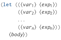
which can be thought of as:
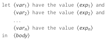
A let expression is simply sytactic sugar for the underlying lambda
application.
A useful example. Let’s stipulate x (outside of let) is 5. Then, the
following expression evaluates to 38.
(+ (let ((x 3))
     (+ x (* x 10)))
   x)
Similarly, if x in the next expression is given as 2, the following expression
evaluates to 12.
(let ((x 3)
      (y (+ x 2)))
  (* x y))
Procedures as General Methods
To find the roots of a continuous function for which we know two values with opposite signs, we can utilise the biscetion method or half-interval method. It is implemented in the following procedure:
(define (search f neg-point pos-point)
  (let ((midpoint (average neg-point pos-point)))
    (if (close-enough? neg-point pos-point)
        midpoint
        (let ((test-value (f midpoint)))
          (cond ((positive? test-value)
                 (search f neg-point midpoint))
                ((negative? test-value)
                 (search f midpoint pos-point))
                (else midpoint))))))

(define (close-enough? x y)
  (< (abs (- x y)) 0.001))

(define (average x y)
  (/ (+ x y) 2))

;; We need to ensure that values of opposite signs are the only valid input,
;; hence we use the following procedure to output an error if that is not the
;; case:

(define (half-interval-method f a b)
  (let ((a-value (f a))
        (b-value (f b)))
    (cond ((and (negative? a-value) (positive? b-value))
           (search f a b))
          ((and (negative? b-value) (positive? a-value))
           (search f b a))
          (else
           (error "Values are not of opposite sign" a b)))))

(half-interval-method sin 2.0 4.0)
;; 3.14111328125
Exercise 1.35
Show that the golden ratio \(\phi\) (Section 1.2.2) is a fixed point of the
transformation \(x \mapsto 1 + \frac{1}{x}\), and use this fact to compute
\(\phi\) by means of the fixed-point procedure.
(define tolerance 0.00001)

(define (fixed-point f first-guess)
  (define (close-enough? v1 v2)
    (< (abs (- v1 v2)) tolerance))
  (define (try guess)
    (let ((next (f guess)))
      (if (close-enough? guess next)
          next
          (try next))))
  (try first-guess))

(define (golden-ratio x)
  (fixed-point (lambda (x) (+ 1 (/ 1 x)))
               1.0))

(golden-ratio 200)
;; 1.6180327868852458
Exercise 1.36
Modify fixed-point so that it prints the sequence of approximations it
generates, using the newline and display primitives shown in Exercise 1.22.
Then find a solution to \(x^x = 1000\) by finding a fixed point of \(x
\mapsto log(1000)/ log(x)\). (Use Scheme’s primitive log procedure, which
computes natural logarithms.) Compare the number of steps this takes with and
without average damping. (Note that you cannot start fixed-point with a guess
of 1, as this would cause division by \(log(1) = 0\).)
(define tolerance 0.00001)

(define (fixed-point f first-guess)
  (define (close-enough? v1 v2)
    (< (abs (- v1 v2)) tolerance))
  (define (try guess)
    (display guess)
    (newline)
    (let ((next (f guess)))
      (if (close-enough? guess next)
          next
          (try next))))
  (try first-guess))

(define (xtothex1k x)
  (fixed-point (lambda (x) (/ (log 1000) (log x)))
               2))
Exercise 1.37
Consider the infinite continues fraction:
and its approximation:
Define a procedure cont-frac such that evaluating (cont-frac n d k) computes
the value of the k-term finite continued fraction. Check your procedure by
approximating \(\frac{1}{\phi}\) using
(cont-frac (lambda (i) 1.0)
           (lambda (i) 1.0)
           k)
for successive values of k. How large must you make k in order to get an
approximation that is accurate to 4 decimal places?
(define (cont-frac n d k)

  (define (rec step)
    (if (= step k)
        (/ (n k) (d k))
        (/ (n step) (+ (d step) (rec (+ step 1))))))
  (rec 0))

(cont-frac (lambda (x) 1.)
           (lambda (x) 1.)
           10)

(define (phi-approx steps)
  (/ 1. (cont-frac (lambda (x) 1.)
                   (lambda (x) 1.)
                   steps)))

;; true value of phi: 1.618033
(phi-approx 1);; 2
(phi-approx 5);; 1.625
(phi-approx 9) ;; 1.6181
(phi-approx 10) ;; 1.617977 - good enough
(phi-approx 11);; 1.61805555 - technically not
(phi-approx 12);; 1.618025 - that's perfect

;; have just written a recursive procedure
;; now let's try an iterative one

(define (cont-frac-iter n d k)
  (define kth-fraction (/ (n k) (d k)))
  ;; start with the k-th term, decrement i each time
  (define (iter i acc)
    (if (= i 0)
        acc
        (iter (- i 1) (/ (n i) (+ acc (d i))))))
  (iter k kth-fraction))

(define (phi-approx-iter steps)
  (/ 1. (cont-frac-iter (lambda (x) 1.) (lambda (x) 1.) steps)))

(phi-approx-iter 10) ;; converges to four decimal places after same number of steps
Exercise 1.38
In 1737, the Swiss mathematician Leonhard Euler published a memoir De Fractionibus Continuis, which included a continued fraction expansion for \(e-2\), where e is the base of the natural logarithms. In this fraction, the \(N_{i}\) are all 1, and the \(D_{i}\) are successively 1, 2, 1, 1, 4, 1, 1, 6, 1, 1, 8, … Write a program that uses your cont-frac procedure from Exercise 1.37 to approximate \(e\), based on Euler’s expansion.
;; take the iterative version
(define (cont-frac n d k)
  (define kth-fraction (/ (n k) (d k)))
  ;; start with the k-th term, decrement i each time
  (define (iter i acc)
    (if (= i 0)
        acc
        (iter (- i 1) (/ (n i) (+ acc (d i))))))
  (iter k kth-fraction))

(define (euler steps)
  (+ 2. (cont-frac (lambda (x) 1)
                   (lambda (x)
                     ;; for 2 and every third number therefater
                     ;; (remainder x 3) evaluates to 2
                     (if (= (remainder x 3) 2)
                         ;; then we need the nearest even integer
                         (/ (+ x 1) 1.5)
                         1))
                   steps)))
Exercise 1.39
Now, we use cont-frac to compute J.H. Lambert’s continued fraction
representation of the tangent function:
;; take the iterative version
(define (cont-frac n d k)
  (define kth-fraction (/ (n k) (d k)))
  ;; start with the k-th term, decrement i each time
  (define (iter i acc)
    (if (= i 0)
        acc
        (iter (- i 1) (/ (n i) (+ acc (d i))))))
  (iter k kth-fraction))

(define (tan-cf angle steps)
  (cont-frac (lambda (i) (if (= i 1)
                             angle
                             (- (square angle))))
             (lambda (i) (- (* i 2) 1))
             steps))

(tan-cf 30. 1000)
;; -6.405331196646245

;; a version from the internet using let where the square is
;; only calculated once
(define (tan-cf-better angle steps)
  (let ((a (- (square angle))))
    (cont-frac (lambda (i) (if (= i 1) angle a))
               (lambda (i) (- (* i 2) 1))
               steps)))

(tan-cf-better 30. 1000)
;; -6.405331196646245
Procedures as Returned Values
As a first useful example of a useful procedure returning another procedure, the authors mention average damping, a convergence acceleration technique:
(define (average-damp f)
  (lambda (x) (average x (f x))))
Using this, you can reformulate the sqrt procedure from above in very
expressive form:
;; remember fixed-point from earlier
(define tolerance 0.00001)
(define (fixed-point f first-guess)
  (define (close-enough? v1 v2)
    (< (abs (- v1 v2)) tolerance))
  (define (try guess)
    (let ((next (f guess)))
      (if (close-enough? guess next)
          next
          (try next))))
  (try first-guess))

(define (sqrt x)
  (fixed-point (average-damp (lambda (y) (/ x y)))
               1.0))

(define (cube-root x)
  (fixed-point (average-damp (lambda (y) (/ x (square y))))
               1.0))
The derivative of a function is defined as:
In Scheme, the authors express this as follows:
(define (deriv g)
  (lambda (x)
    (/ (- (g (+ x dx)) (g x))
       dx)))
(define dx 0.00001)
Now, you can express Newton’s method, \(g(x) = 0\) is a fixed point of the function , where
Again, in Scheme, you can express this like so:
(define (newton-transform g)
  (lambda (x)
    (- x (/ (g x) ((deriv g) x)))))

(define (newtons-method g guess)
  (fixed-point (newton-transform g) guess))

;; now we can find the square roots of f(x) = y^2 - x using Newton's method
(define (sqrt x)
  (newtons-method (lambda (y) (- (square y) x))
                  1.0))
This can be generalised even further by realising that both Newton’s method and
the method using fixed-point were doing almost the same, i.e. both begin with
a function and end with finding the fixed point of a transformation of that
initial function. In Scheme:
;; g is some function
;; transform is its transformation
;; and guess is where the procedure starts
(define (fixed-point-of-transform g transform guess)
  (fixed-point (transform g) guess))

;; using this, you can rewrite the functions from above
(define (sqrt x)
  (fixed-point-of-transform (lambda (y) (/ x y))
                            average-damp
                            1.0))

(define (sqrt x)
  (fixed-point-of-transform (lambda (y) (- (square y) x))
                            newton-transform
                            1.0))
Programming languages impose restrictions on the ways computational elements can be manipulated. Those elements to which the fewest restrictions are applied are called first-class elements. They may:
- be named by variables
- be passed as arguments to procedures
- be returned as the results of the procedures
- be included in data structures
Lisp treats procedures as first-class elements, hence Lisp is a functional programming language. This, however, the authors claim poses challenges for efficient implementation, but creates “enormous” (p. 103) gains in expressive power.
Exercise 1.40
Define a procedure cubic that can be used together with the newtons-method procedure in expressions of the form:
(newtons-method (cubic a b c) 1)
to approximate zeros of the cubic
(define tolerance 0.00001)
(define (fixed-point f first-guess)
  (define (close-enough? v1 v2)
    (< (abs (- v1 v2)) tolerance))
  (define (try guess)
    (let ((next (f guess)))
      (if (close-enough? guess next)
          next
          (try next))))
  (try first-guess))

(define (deriv g)
  (lambda (x)
    (/ (- (g (+ x dx)) (g x))
       dx)))
(define dx 0.00001)

(define (newton-transform g)
  (lambda (x)
    (- x (/ (g x) ((deriv g) x)))))

(define (newtons-method g guess)
  (fixed-point (newton-transform g) guess))

(define (cubic a b c)
  (lambda (x) (+ (cube x) (* a (square x)) (* b x) c)))

(newtons-method (cubic 1 2 3) 1)
;; -1.2756822036498454
Exercise 1.41
Define a procedure double that takes a procedure of one argument as argument and
returns a procedure that applies the original procedure twice. For example, if
inc is a procedure that adds 1 to its argument, then (double inc) should be
a procedure that adds 2. What value is returned by
(((double (double double)) inc) 5)?
(define (inc i)
  (+ i 1))

(define (double f)
  (lambda (x) (f (f x))))

(((double (double double)) inc) 5)
;; 21
Exercise 1.42
Let \(f\) and \(g\) be two one-argument functions. The composition \(f\)
after \(g\) is defined to be the function \(x \mapsto f(g(x))\). Define a
procedure compose that implements composition. For example, if inc is a
procedure that adds 1 to its argument, ((compose square inc) 6) evaluates
to 49.
(define (inc i)
  (+ i 1))

(define (compose f g)
  (lambda (x) (f (g x))))

((compose square inc) 6)
;; 49
Exercise 1.43
If f is a numerical function and \(n\) is a positive integer, then we can form
the \(n^{th}\) repeated application of \(f\) , which is defined to be the
function whose value at \(x\) is \(f(f(…(f(x))…))\). For example, if
\(f\) is the function , then the \(n^{th}\) repeated
application of \(f\) is the function \(x \mapsto x + n\). If \(f\) is the
operation of squaring a number, then the \(n^{th}\) repeated application of
\(f\) is the function that raises its argument to the \(2^{n}\) -th power.
Write a procedure that takes as inputs a procedure that computes \(f\) and a
positive integer \(n\) and returns the procedure that computes the
\(n^{th}\) repeated application of \(f\). Your procedure should be able to
be used as follows: ((repeated square 2) 5) evaluates to 625.
;; primitives
(define (compose f g)
  (lambda (x) (f (g x))))

(define (identity x) x)

;; recursive
(define (repeated f n)
  (if (= n 1)
      f
      (compose f (repeated f (- n 1)))))

;; iterative
(define (repeated-iter f n)
  (define (iter n result)
    (if (< n 1)
        result
        (iter (- n 1) (compose f result))))
  (iter n identity))

((repeated square 3) 5)
;; 390625

((repeated-iter square 3) 5)
;; 390625
Exercise 1.44
The idea of smoothing a function is an important concept in signal processing.
If \(f\) is a function and \(dx\) is some small number, then the smoothed
version of \(f\) is the function whose value at a point \(x\) is the average
of f \((x − dx)\), \(f (x)\), and \(f (x +dx)\). Write a procedure
smooth that takes as input a procedure that computes \(f\) and returns a
procedure that computes the smoothed \(f\). It is sometimes valuable to
repeatedly smooth a function (that is, smooth the smoothed function, and so on)
to obtain the n-fold smoothed function. Show how to generate the n-fold smoothed
function of any given function using smooth and repeated from Exercise 1.43.
;; needed primitives
(define (deriv g)
  (lambda (x)
    (/ (- (g (+ x dx)) (g x))
       dx)))
(define dx 0.00001)

(define (average x y z)
  (/ (+ x y z) 3))

(define (smooth f)
  (lambda (x) (average (- x dx) x (+ x dx))))

(define (compose f g)
  (lambda (x) (f (g x))))

(define (repeated f n)
  (if (= n 1)
      f
      (compose f (repeated f (- n 1)))))

(define (n-fold-smooth f n)
  (repeated smooth n) f)
Exercise 1.45
Unfortunately, the average-dump process does not work for fourth roots — a
single average damp is not enough to make a fixed-point search for \(y \mapsto
x/y^{3}\) converge. On the other hand, if we average damp twice (i.e., use the
average damp of the average damp of \(y \mapsto x/y^{3}\)) the fixed-point
search does converge. Do some experiments to determine how many average damps
are required to compute \(n_{th}\) roots as a fixed-point search based upon
repeated average damping of \(y \mapsto x/y_{n - 1}\). Use this to implement
a simple procedure for computing \(n_{th}\) roots using fixed-point,
average-damp, and the repeated procedure
(define (average x y)
  (/ (+ x y) 2.0))

(define (average-damp f)
  (lambda (x) (average x (f x))))

(define tolerance 0.00001)

(define (fixed-point f first-guess)
  (define (close-enough? v1 v2)
    (< (abs (- v1 v2)) tolerance))
  (define (try guess)
    (let ((next (f guess)))
      (if (close-enough? guess next)
          next
          (try next))))
  (try first-guess))

(define (repeated f n)
  (if (= n 1)
      f
      (compose f (- n 1)) x))

;; from solutions
(define (get-max-pow n)
  (define (iter p r)
    (if (< (- n r) 0)
        (- p 1)
        (iter (+ p 1) (* r 2))))

  (iter 1 2))

(define (pow b p)
  (define (even? x)
    (= (remainder x 2) 0))

  (define (sqr x)
    (* x x))

  (define (iter res a n)
    (if (= n 0)
        res
        (if (even? n)
            (iter res (sqr a) (/ n 2))
            (iter (* res a) a (- n 1)))))

  (iter 1 b p))

(define (nth-root n x)
  (fixed-point ((repeated average-damp (get-max-pow n))
                (lambda (y) (/ x (pow y (- n 1)))))
               1.0))
Exercise 1.46
Several of the numerical methods described in this chapter are instances of an
extremely general computational strategy known as iterative improvement.
Iterative improvement says that, to compute something, we start with an initial
guess for the answer, test if the guess is good enough, and otherwise improve
the guess and continue the process using the improved guess as the new guess.
Write a procedure iterative-improve that takes two procedures as arguments: a
method for telling whether a guess is good enough and a method for improving a
guess. iterative-improve should return as its value a procedure that takes a
guess as argument and keeps improving the guess until it is good enough. Rewrite
the sqrt procedure and the fixed-point procedure in terms of
iterative-improve.
(define (iterative-improve good-enough? improve)
  (lambda (guess)
    (if (good-enough? guess)
        guess
        ((iterative-improve good-enough? improve) (improve guess)))))

(define (close-enough? v1 v2)
  (< (abs (- v1 v2)) tolerance))

(define (fixed-point f first-guess)
  ((iterative-improve
    (lambda (x) (close-enough? x (f x)))
    f)
   first-guess))

(define (sqrt x)
  ((iterative-improve
    (lambda (y)
      (< (abs (- (square y) x))
         0.0001))
    (lambda (y)
      (average y (/ x y))))
   1.0))
Building Abstraction with Data
The authors introduce some critical notions in the opening to chapter two:
- compound data is simply the result of a combination of data objects, i.e. the combination of a numerator and a denominator to represent a rational number
- closure is the notion that the “glue” used for combining data objects should allow not only for combining primitive data object (such as integers) but compound data objects as well.
- compound data objects can serve as conventional interfaces for combining program modules
- symbolic expressions are data whose elementary parts can be any symbol rather than only numbers.
- data-directed programming is a technique that allows different data representations to be designed in isolation to then be combined additively (i.e. without modification)
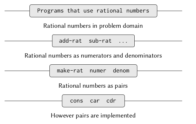
Introduction to Data Abstraction
The basic idea of data abstraction is to structure the programs that are to use compound data objects so that they operate on “abstract data.” That is, our programs should use data in such a way as to make no assumptions about the data that are not strictly necessary for performing the task at hand. (Abelson and Sussman 2002, 112)
Concrete data representations, on the other hand, are defined independent of the programs using the data. The interface between abstract data and its concrete representations are a set of procedures called selectors and constructors that implement the abstract data in terms of its concrete representation.
In the case of rational numbers a constructor (make-rat n d) returns the
rational number whose numerator is the integer n and whose denominator is the
integer d. The selectors (numer x) and (denom x) return the numerator and
denominator respectively. We leave them undefined for now. If we had them,
however (wishful thinking) the following relations would allow us to do all
sorts of things with rational numbers:
as procedures they look as follows:
#lang sicp
(define (add-rat x y)
  (make-rat (+ (* (numer x) (denom y))
               (* (numer y) (denom x)))
            (* (denom x) (denom y))))

(define (sub-rat x y)
  (make-rat (- (* (numer x) (denom y))
               (* (numer y) (denom x)))
            (* (denom x) (denom y))))

(define (mul-rat x y)
  (make-rat (* (numer x) (numer y))
            (* (denom x) (denom y))))

(define (div-rat x y)
  (make-rat (* (numer x) (denom y))
            (* (denom x) (numer y))))

(define (equal-rat? x y)
  (= (* (numer x) (denom y))
     (* (numer y) (denom x))))
Pairs
Pairs are the a compound data structure provided by Lisp. They are constructed and selected from as follows:
#lang sicp
(define x (cons 1 2))
(car x)
;; 1
(cdr x)
;; 2
;; we can also combine pairs with pairs
(define y (cons 3 4))
(define z (cons x y))
(car (car z))
;; 1
(car (cdr z))
;; 3
(car z)
;; (1 . 2)
Now rational numbers can be easily represented:
#lang sicp
;; (define (make-rat n d) (cons n d))
;; the rational numbers are not reduced. In order to do that, we have to change
;; make-rat
(define (make-rat n d)
  (let ((g (gcd n d)))
    (cons (/ n g) (/ d g))))

(define (numer x) (car x))
(define (denom x) (cdr x))
;; to print them we can use
(define (print-rat x)
  (newline)
  (display (numer x))
  (display "/")
  (display (denom x)))
;; let's try everything out
(define one-half (make-rat 1 2))
(print-rat one-half)
;; 1/2
(define (add-rat x y)
  (make-rat (+ (* (numer x) (denom y))
               (* (numer y) (denom x)))
            (* (denom x) (denom y))))
(print-rat (add-rat one-half one-half))
;; formerly 4/4, now 1/1
Exercise 2.1
Define a better version of make-rat that handles both positive and negative
arguments. make-rat should normalize the sign so that if the rational number
is positive, both the numerator and denominator are positive, and if the
rational number is negative, only the numerator is negative.
#lang sicp
(define (make-rat n d)
  (let ((g ((if (< d 0) - +) (abs (gcd n d)))))
    (cons (/ n g) (/ d g))))

(make-rat 18 -9)
;; (-2 . 1)
Abstraction Barriers
Exercise 2.2
Consider the problem of representing line segments in a plane. Each segment is
represented as a pair of points: a starting point and an ending point. Define a
constructor make-segment and selectors start-segment and end-segment that
define the representation of segments in terms of points. Furthermore, a point
can be represented as a pair of numbers: the x coordinate and the y coordinate.
Accordingly, specify a constructor make-point and selectors x-point and
y-point that define this representation. Finally, using your selectors and
constructors, define a procedure midpoint-segment that takes a line segment as
argument and returns its midpoint (the point whose coordinates are the average
of the coordinates of the endpoints). To try your procedures, you’ll need a way
to print points:
#lang sicp
(define (make-point x y)
  (cons x y))
(define (x-point p)
  (car p))
(define (y-point p)
  (cdr p))

(define (make-segment p1 p2)
  (cons p1 p2))
(define (start-segment s)
  (car s))
(define (end-segment s)
  (cdr s))

(define (print-point p)
  (newline)
  (display "(")
  (display (x-point p))
  (display ",")
  (display (y-point p))
  (display ")"))

(define (average x y)
  (/ (+ x y) 2))

(define point1 (make-point 3 3 ))
(define point2 (make-point 1 1 ))

(define segment (make-segment point1 point2))

(define (midpoint-segment s)
  (let ((x-point (car s)))
    (let ((y-point (cdr s)))
      (cons (average (car x-point) (car y-point))
            (average (cdr x-point) (cdr y-point))))))

;;(midpoint-segment segment)
;; (2 . 2)
Exercise 2.3
#lang sicp
;; Point
(define (make-point x y) (cons x y))
(define (x-point p) (car p))
(define (y-point p) (cdr p))

;; Rectangle - 1st implementation
(define (make-rect bottom-left top-right)
  (cons bottom-left top-right))

;; "Internal accessors", not to be used directly by clients.  Not sure
;; how to signify this in scheme.
(define (bottom-left rect) (car rect))
(define (bottom-right rect)
  (make-point (x-point (cdr rect))
              (y-point (car rect))))
(define (top-left rect)
  (make-point (x-point (car rect))
              (y-point (cdr rect))))
(define (top-right rect) (cdr rect))

(define (width-rect rect)
  (abs (- (x-point (bottom-left rect))
          (x-point (bottom-right rect)))))
(define (height-rect rect)
  (abs (- (y-point (bottom-left rect))
          (y-point (top-left rect)))))

;; Public methods.
(define (area-rect rect)
  (* (width-rect rect) (height-rect rect)))
(define (perimeter-rect rect)
  (* (+ (width-rect rect) (height-rect rect)) 2))


;; Testing:
(define r1 (make-rect (make-point 1 1)
                     (make-point 3 7)))
(area-rect r1)
(perimeter-rect r1)

;; 12
;; 16

;; Rectangle - 2nd implementation
;; assuming, not checking width, height > 0.
(define (make-rect-alt bottom-left width height)
  (cons bottom-left (cons width height)))

(define (height-rect-alt rect) (cdr (cdr rect)))
(define (width-rect-alt rect) (car (cdr rect)))

;; area and perimeter ops remain unchanged.  The internal methods from
;; the first implementation won't work now.

;; Testing:
(define r2 (make-rect-alt (make-point 1 1) 2 6))

(define (area-rect-alt rect)
  (* (width-rect-alt rect) (height-rect-alt rect)))
(define (perimeter-rect-alt rect)
  (* (+ (width-rect-alt rect) (height-rect-alt rect)) 2))

(area-rect-alt r2)
(perimeter-rect-alt r2)
;; 12
;; 16